01 Task File
Explore Files
# !gcloud storage ls gs://wqu-cv-course-datasets
# gcloud storage cp gs://wqu-cv-course-datasets/ptoject1.tar.gz  --no clobber
# !tar --skip-old-files -xzf project1.tar.gz
Task 1.1.11: Following the pattern of data_dir, assign the path to the multi-class training data to train_dir.
data_dir = os.path.join("data_p1", "data_multiclass")
train_dir = os.path.join(data_dir, "train")

print("data_dir class:", type(data_dir))
print("Data directory:", data_dir)
print()
print("train_dir class:", type(train_dir))
print("Training data directory:", train_dir)
Result:
data_dir class: <class 'str'>
Data directory: data_p1/data_multiclass

train_dir class: <class 'str'>
Training data directory: data_p1/data_multiclass/train
Task 1.1.12: Create a list of the contents of train_dir, and assign the result to class_directories.
class_directories = os.listdir(train_dir)

print("class_directories type:", type(class_directories))
print("class_directories length:", len(class_directories))
print(class_directories)
Result:
class_directories type: <class 'list'>
class_directories length: 8
['hog', 'blank', 'monkey_prosimian', 'antelope_duiker', 'leopard', 'civet_genet', 'bird', 'rodent']
It looks like our training directory contains 8 subdirectories. Judging by their names, each contains the images for one of the classes in our dataset.
Task 1.1.13: Complete the for loop so that class_distributions_dict contains the name of each subdirectory as its keys and the number of files in each subdirectory as its values.
class_distributions_dict = {}

for subdirectory in class_directories:
   dir = os.path.join(train_dir, subdirectory)
   files = os.listdir(dir)
   num_files = len(files)
   class_distributions_dict[subdirectory] = num_files

class_distributions = pd.Series(class_distributions_dict)

print("class_distributions type:", type(class_distributions))
print("class_distributions shape:", class_distributions.shape)
print(class_distributions)
Result:
class_distributions type: <class 'pandas.core.series.Series'>
class_distributions shape: (8,)
hog                  978
blank               2213
monkey_prosimian    2492
antelope_duiker     2474
leopard             2254
civet_genet         2423
bird                1641
rodent              2013
dtype: int64
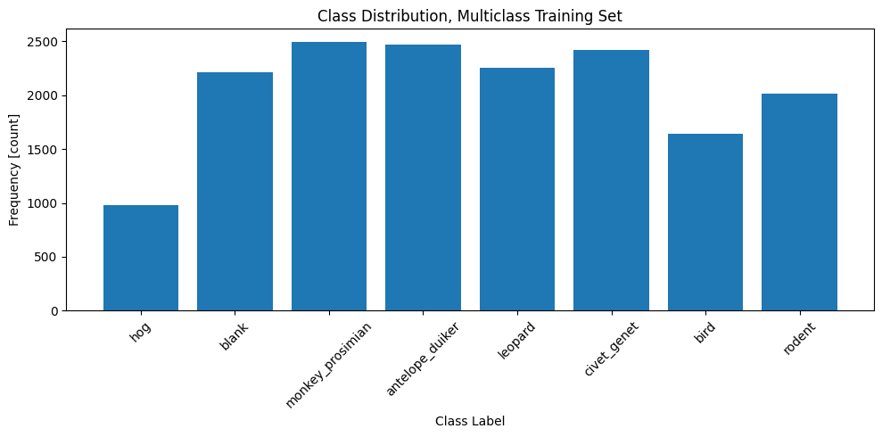
Task 1.1.14: Create a bar chart from class_distributions.
# Create a bar plot of class distributions
fig, ax = plt.subplots(figsize=(10, 5))

# Plot the data
ax.bar(class_distributions.index, class_distributions.values) # Write your code here
ax.set_xlabel("Class Label")
ax.set_ylabel("Frequency [count]")
ax.set_title("Class Distribution, Multiclass Training Set")
plt.xticks(rotation=45)
plt.tight_layout()
plt.show()
Load Images
# Define path for hog image
hog_image_path = os.path.join(train_dir, "hog", "ZJ000072.jpg")

# Define path for antelope image
antelope_image_path = os.path.join(train_dir, "antelope_duiker", "ZJ002533.jpg")

print("hog_image_path type:", type(hog_image_path))
print(hog_image_path)
print()
print("antelope_image_path type:", type(antelope_image_path))
print(antelope_image_path)
Result:
hog_image_path type: <class 'str'>
data_p1/data_multiclass/train/hog/ZJ000072.jpg

antelope_image_path type: <class 'str'>
data_p1/data_multiclass/train/antelope_duiker/ZJ002533.jpg
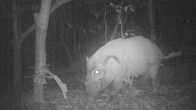
To load these images, we'll use the Pillow library (aka PIL), which comes with lots of tools for image processing. We'll start with the hog.
hog_image_pil = Image.open(hog_image_path)

print("hog_image_pil type:", type(hog_image_pil))
hog_image_pil
hog_image_pil type: <class 'PIL.JpegImagePlugin.JpegImageFile'>
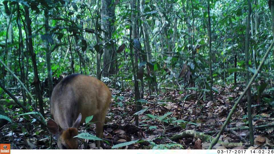
Task 1.1.15: Use PIL to open antelope_image_path.
antelope_image_pil = Image.open(antelope_image_path)

print("antelope_image_pil type:", type(antelope_image_pil))
antelope_image_pil
antelope_image_pil type: <class 'PIL.JpegImagePlugin.JpegImageFile'>
Let's keep using PIL to explore further, looking at their .size and .mode attributes. Again, we'll start with the hog and then do the antelope.
# Get image size
hog_image_pil_size = hog_image_pil.size

# Get image mode
hog_image_pil_mode = hog_image_pil.mode

# Print results
print("hog_image_pil_size class:", type(hog_image_pil_size))
print("hog_image_pil_size length:", len(hog_image_pil_size))
print("Hog image size:", hog_image_pil_size)
print()
print("hog_image_pil_mode class:", type(hog_image_pil_mode))
print("Hog image mode:", hog_image_pil_mode)
Result:
hog_image_pil_size class: <class 'tuple'>
hog_image_pil_size length: 2
Hog image size: (640, 360)

hog_image_pil_mode class: <class 'str'>
Hog image mode: L
Task 1.1.16: Get the .size and .mode attributes from antelope_image_pil and assign the results to antelope_image_pil_size and antelope_image_pil_mode, respectively.
# Get image size
antelope_image_pil_size = antelope_image_pil.size

# Get image mode
antelope_image_pil_mode = antelope_image_pil.mode

# Get image mode
print("antelope_image_pil_size class:", type(antelope_image_pil_size))
print("antelope_image_pil_size length:", len(antelope_image_pil_size))
print("Antelope image size:", antelope_image_pil_size)
print()
print("antelope_image_pil_mode class:", type(antelope_image_pil_mode))
print("Antelope image mode:", antelope_image_pil_mode)
Result:
antelope_image_pil_size class: <class 'tuple'>
antelope_image_pil_size length: 2
Antelope image size: (960, 540)

antelope_image_pil_mode class: <class 'str'>
Antelope image mode: RGB
Looking at these attributes, we can confirm that there are two differences between our images.
Mode: The hog image is in grayscale (
mode="L"), while the antelope image is in color mode (mode="RGB").Size: The hog images is smaller than the antelope image.
These differences are important because all the images in our dataset must have the same size and mode before we can use them to train a model.
Load Tensors
hog_tensor = transforms.ToTensor()(hog_image_pil)

print("hog_tensor type:", type(hog_tensor))
print("hog_tensor shape:", hog_tensor.shape)
print("hog_tensor dtype:", hog_tensor.dtype)
print("hog_tensor device:", hog_tensor.device)
Result:
hog_tensor type: <class 'torch.Tensor'>
hog_tensor shape: torch.Size([1, 360, 640])
hog_tensor dtype: torch.float32
hog_tensor device: cpu
Task 1.1.17: Convert antelope_image_pil to a tensor and assign the result to antelope_tensor.
antelope_tensor = transforms.ToTensor()(antelope_image_pil)

print("antelope_tensor type:", type(antelope_tensor))
print("antelope_tensor shape:", antelope_tensor.shape)
print("antelope_tensor dtype:", antelope_tensor.dtype)
print("antelope_tensor device:", antelope_tensor.device)
Result:
antelope_tensor type: <class 'torch.Tensor'>
antelope_tensor shape: torch.Size([3, 540, 960])
antelope_tensor dtype: torch.float32
antelope_tensor device: cpu
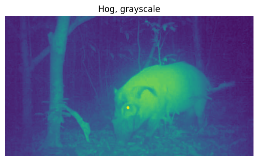
In addition to height and width, image files generally come with color channels. A color channel holds information about the intensity of a specific color for each pixel in an image. Because our hog image is grayscale, there's only one color to represent: gray. In fact, if we extract the values from the gray channel in hog_tensor and plot them, we end up with the same image we saw in the last section.
# Create figure with single axis
fig, ax = plt.subplots(1, 1)

# Plot gray channel of hog_tensor
ax.imshow(hog_tensor[0, :, :])

# Turn off x- and y-axis
ax.axis("off")

# Set title
ax.set_title("Hog, grayscale");
While the hog image is grayscale, the antelope image is in color. Its mode is RGB, which stands red, green, and blue. Each of these colors has its own channel in the image. That's where the 3 in the antelope_tensor shape [3, 540, 960] comes from. We can extract the values for each channel using our slicing skills and plot them side-by-side.
Task 1.1.18: Complete the code below to plot the red, green, and blue channels of antelope_tensor.
# Create figure with 3 subplots
fig, (ax0, ax1, ax2) = plt.subplots(1, 3, figsize=(15, 5))

# Plot red channel
red_channel = antelope_tensor[0, :, :]
ax0.imshow(red_channel, cmap="Reds")
ax0.set_title("Antelope, Red Channel")
ax0.axis("off")

# Plot green channel
green_channel = ...


# Plot blue channel
blue_channel = ...


plt.tight_layout();
The key takeaway is that the dimensions for an image tensor are always (C x H x W), channel by height by width.
Task 1.1.19: Calculate the minimum and maximum values of antelope_tensor and assign the results to max_channel_values and min_channel_values, respectively.
max_channel_values = ...
min_channel_values = ...

print("max_channel_values class:", type(max_channel_values))
print("max_channel_values shape:", max_channel_values.shape)
print("max_channel_values data type:", max_channel_values.dtype)
print("max_channel_values device:", max_channel_values.device)
print("Max values in antelope_tensor:", max_channel_values)
print()
print("min_channel_values class:", type(min_channel_values))
print("min_channel_values shape:", min_channel_values.shape)
print("min_channel_values data type:", min_channel_values.dtype)
print("min_channel_values device:", min_channel_values.device)
print("Min values in antelope_tensor:", min_channel_values)
We can see that the values in the tensor range from 0 to 1. 0 means that the color intensity at a particular pixel is 0%; 1 means intensity is 100%.
Task 1.1.20: Calculate the mean values of the separate color channels in antelope_tensor and assign the result to mean_channel_values.
mean_channel_values = ...

print("mean_channel_values class:", type(mean_channel_values))
print("mean_channel_values shape:", mean_channel_values.shape)
print("mean_channel_values dtype:", mean_channel_values.dtype)
print("mean_channel_values device:", mean_channel_values.device)
print("Mean channel values in antelope_tensor (RGB):", mean_channel_values)
Key Points:
here are the key discoveries we've made about our dataset in this lesson:
Our dataset is organized into folders. We have data for a binary classification model and a multi-class model. In both cases, the training data is divided into subdirectories, one for each class.
The images in our dataset come in different sizes.
The images in our dataset come in different modes (grayscale and RGB).
When we convert our images from PIL to tensors, their values range from
0to1.


